Final Project: Suitability Map of Worst Locations For Child-Bearing

Intro

As a geographer and a cartographer, I wanted to focus on the cultural aspects of different geographical locations in relation to infant health. The question I had at hand was which countries would be the worst for me to start and maintain a family with children so that I could avoid them. I love the United States but I wanted to try something different and my personal goal has always been to live in beautiful Ethiopia because I had an apartment in the Little Ethiopian District of Los Angeles and I felt that the culture was vividly rich and the food was beyond delicious. This project was a goal to determine whether or not Ethiopia would be a suitable or viable location to start my family. I was thinking of factors that would lead to a proper health care system for my children to be born into, as well as a location that would provide equal opportunities for my newly established family. I decided to look at the most up-to-date GINI and Infant Mortality Rates because I wanted to find the worst locations for child bearing. This can be useful for individuals that plan on moving to another country to start a family because they can see which country is most suitable for their child- bearing needs. This GIS vector spatial analysis adds value to the given information and to my topic of choice because it can provide the suitability output with two crucial factors. In analyzing the information at hand, I am able to create a map that will provide suitability rankings of different countries in the world and can broaden my perspective on which countries I would want to avoid moving to.


Methods

To begin the creation of the suitability map, data acquisition from CIA.gov was needed for the Infant Mortality Rates and Nation Master.com provided the most up-to-date GINI index of the world’s countries. I chose the GINI index and its corresponding coefficients since it was a good indicator for distribution of income or wealth within a country. The GINI index incorporated many factors that have “found application in the study of inequalities in disciplines as diverse as sociology, economics, health science, ecology, chemistry and engineering.” (Wikipedia.org) It has found many uses because it is a good indicator on how well the infrastructure is in that given country. The Infant Mortality Rate (IMR) was used because this can give me a good indication of whether or not the country has a hospitable, safe and clean environment for children to be born in. The Microsoft Excel program was used to sort the data and then afterwards, a DBF could be created in ArcCatalog for the transfer into ArcGIS. With the Excel program, the fields of Infant Morality Rates and GINI index were able to be on the same spread sheet. The data from the excel spread sheet was used to create a join with the attribute table of the world shape file. Afterwards, I opened the attribute table in ArcGIS to add a new field. This new field would become the new map of suitability and to calculate this, the equation (INFANT MORTALITY RATE x .6 + GINI Index X .4) was used. The given weighted variables for IMR and GINI were concluded by examining how the IMR is more important in this suitability map because our main concern is to determine the worst location for child birth and not solely concerned with inequality. Although the GINI index field is very vital since it is a main factor that leads to the emergence of a low or high IMR, it should be noted that the IMR focuses more directly to the topic question and map theme at hand. Infant Mortality Rates was given an arbitrary value of .6 while the GINI was given .40. One field was given more weight than the other due to research that shows that although GINI coefficient reflect inequality ratings of a country and can be directly related to the Infant Mortality Rates, ultimately the Infant Mortality Rates are more precise in the final suitability map that determines the worst places for child-bearing.
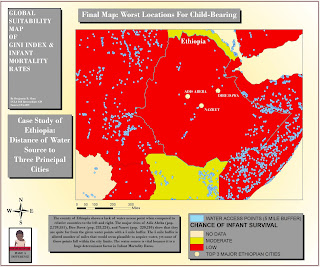
After the suitability map with the two factors of GINI and IMR were created, I wanted to focus more in-depth on the country of Ethiopia as a case study. This will help me in determining why Ethiopia was ranked in certain position on the final suitability map and this needed data acquisition from UCLA GIS database for water sources. The factor of water sources is vital in influencing IMR because one of the main causes of infant death is the lack of water. “Traditionally, the most common cause worldwide was dehydration” and with the given water point data, a 5 mile buffer can be created using the buffer tool in the Arc Toolbox in ArcGIS to see how accessible water is in three major cities in Ethiopia.


Results


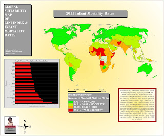
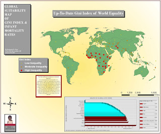
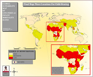
The maps support the research and display values that logically correlate with each other. The IMR Map reported that the countries within the continent of Africa and the country of Afghanistan had the highest infant mortality rates. The high number of Infant deaths for these top tier IMR countries ranged from 81.41 to 175.90 infant deaths per 1000 live births. The GINI index map reported similar results with the focal point on many African countries falling in the “High Inequality” bracket. Afghanistan also fell within this range. It was rather interesting that Africa had such a high concentration of infant deaths and inequality. It led me to believe my assumption that the lack of equality within a country will result in the lack of resources for infants. The Final Suitability Map was the final output needed to determine which location were bad options for child-bearing. I have realized that the country of Ethiopia would be one of the worst places in the world for child-bearing and I would have to re evaluate my decision on moving there.


Further research on the factors of IMR will show that dehydration was a main cause and a creation of a buffer map of the three major cities in Ethiopia to show their proximity to the water point data would be useful. Looking at Ethiopia itself, it is clear that the country does not have as much access to water as seen by the data acquired for UCLA GIS database. The distance of the water sources were far from the top three major cities leading me to believe that the lack of hydration is a huge problem in the country.


Before reaching my results, there were problems that I had encountered such as the fact that not all countries had accurate information such as: Congo, Democratic Republic of Congo, Botswana, North Korea, United Arab Emirates, and Myanmar. This inaccuracy and lack of information can be due to the lack of infrastructure in the country. The lack of infrastructure would result in the absence of a lot of census information or vital statistics making it hard to acquire all the necessary data. I conclude that some of the more developed countries such as North Korea may not have a lack of infrastructure but rather they would not want their information leaked. Another problem was experienced due to the attempted joins of the excel sheet and the country field on the shape file. I had to cross check all the names to make sure that they were in the proper spelling so that they could be compatible to join. If there was any error in the name, the information would not show up correctly on the map output. This was a tedious task since there were so many countries that needed to be checked and edited.


Conclusion/ Discussion


Looking at the map, most of the countries with the worst ranking for child-bearing are in Africa and this can be due to the low Infant Mortality Rate and the high inequality shown in the GINI index. Another map with the focus on Ethiopia was made in order to show how the vast proximity of major cities to water access plays a role in creating a higher IMR. Water is a very essential factor needed for the survival of young infants and even though the major cities are far from the water sources, there should be some type of infrastructure that can make the process of obtaining water easier. Unfortunately for Ethiopia, they also have high inequality as shown by the GINI index map, which would lead one to assume that the distribution of wealth, income and basic necessities is not fair. The question that I had at hand about analyzing whether or not Ethiopia would be a suitable and safe place for my personal child bearing has proven to be an obvious one. The country of Ethiopia is definitely not a suitable place for child-bearing. The neighboring countries of Kenya and Eritrea are better options and as shown to be more suitable by the final suitability map. It is rather unfortunate that the country of Ethiopia falls into that ranking and would not seem like the best suitable place to start and grow a family in, but I am glad that I was able to produce a suitability map so that I could analyze the country and make a knowledgeable decision.

Sources
http://www.cdc.gov/omhd/amh/factsheets/infant.htm
http://www.dcp2.org/file/66/Disease%20and%20Mortality%20in%20SSA.pdf
CIA.gov
Nationmaster.com
http://en.wikipedia.org/wiki/Infant_mortality
http://en.wikipedia.org/wiki/Gini_coefficient
http://gis.ats.ucla.edu/mapshare/

SPATIAL INTERPOLATION: LA COUNTY RAINFALL IN INCHES

For the final lab, we were given a hypothetical situation where the county of Los Angeles has hired us to conduct a spatial interpolation on precipitation. Many points were gathers and formatted on an excel sheet. In an attempt to cover the entire county, various points from all over Los Angeles were taken. Some discrepancies that I experienced were the total and normal precipitation of the Rolling Hills rain gauge indicator. It showed a discrepancy between the data given from the absent normal precipitation versus the given total levels. The data was then not added from the LADWP.org website hence the missing data close to the bottom of the county. I chose only the data that I felt could be best represented on the map. In addition, the LA Country gauge station map lacks many points in the northern rural portion of the county, just like how the Rolling Hills gauge was not appearing on the normal map on LADWP.org.

Spatial interpolation is a useful tool for extending spatial data and is helpful when funding and time is limited. Through spatial interpolation, sample points are used in order to make a better prediction of the area around the point. When looking at precipitation, spatial interpolation allows the county to make a good estimate on precipitation levels based on a relatively small set of points. The need to gather data from every single point in the county is not necessary; rather the collection of several points that cover the county is adequate. According to Dr. Barnali Dixon from University of South Florida St. Petersburg, her paper “Spatial Interpolation of Rainfall Data Using ArcGIS: A Comparative Study” stated that IDW and Kriging are the most commonly used spatial interpolation methods for estimating rainfall.”

The interpolation maps of Los Angeles County precipitation reveal that most of the county’s levels did not fluctuate too much from the norm. The spatial interpolation processes that I used were IDW and Spline. I felt that the statement from the research of Dr. Barnali Dixon is correct in stating that IDW was a good method for interpolating precipitation. I felt that the IDW was better than the Spline technique that I used. For some odd reason the Spline data showed negative values of the precipitation. At first I thought it had been an error on my behalf, but I soon realized that most people that implemented the Spline methods observed the same results. Also, the concentration of land with below average rainfall is not pronounced in the Spline map and an overall deficiency in rainfall looks as if it is more prominent but I began to think of the negative values and how that would affect the overall map. Honestly, at first I could not really tell the differences between IDW and Spline and why an ArcGIS user would use one over another. But upon further analysis, I feel that the IDW is easier for the map user to interpret the difference. The recent versus normal in IDW shows differences and the maps do not seem to be too different while showing the necessary info. While the Spline method seems to have drastically different maps from normal versus recent. Overall, I felt that IDW does a better job over Spline in precipitation interpolation analysis.

FIRE MAP

The map of the 2009 station fire in Los Angeles County required that we use raster data to create a slope map, a vegetation map, and a final raster calculation of both features. It also required that we needed to find data from outside sources not given to us from the class website. The methods used in the tutorial were useful in my personal lab application. The process of data acquisition a challenging steps. The methods of raster analysis masking and the reclassification of layers helped greatly to understand and create the final map. From previous knowledge, I decided to search the USGS seamless server and seamless viewer page to obtain the DEM information which I can then use to analyze my slope and create a hill shade. The raster masking tool that I used to clip off the unwanted parts of the DEM so that it could focus on just the LA county perimeter proved unnecessary because I ended up zooming into the fire parameters so the masking could not be noticed. The DEM was used to make the hill shade and slope map. The slope data needed to be reclassified accordingly. I also used the information and data from LA GIS Enterprise to get the fire parameters that wreaked havoc in the region on the Angeles National Forest in 2009. I was able to obtain the full extent of the fire information with the amount and area of vegetation burned during a specific time ranging from August to September. I also went to the Census.gov to obtain a tiger file shape file of data to overlap it onto my final map to show which cities and districts bordered the 2009 station fire. They included San Fernando Valley, Pasadena, and South Antelope Valley. The Los Angeles County shape file used for the inset map was obtained from UCLA GIS as a polygon from the website. The FRAP website also gave very relevant information on certain vegetation types that resided in the area. The given information with the vegetation was reclassified according to the ‘new values’ given in the tutorial from the Geog 169 class website so that the similar burn hazard vegetation can be classified together. The vegetation was classified to the appropriate new value level is so it can be classified from a high to low danger rating.
Problems that I encountered was the fact that the FRAP website could easily confuse a user in downloading the wrong type of information. The difference between the tutorial and my own lab tended to confuse me. The different data between the tutorial and within my own lab made it difficult to put together particular methods for solving certain problems. One step in the tutorial stated that you needed to click a radio button to link the layer to an AVI file tended to confuse me when I was doing my own lab because I couldn’t find the buttons. I later realized that it was not necessary. I had trouble confirming layer formats, cell sizes and changes in extent coverage. By working it, I was able to better understand the processes behind the final production and the methods used. I also had trouble with the slope values because the percentage was projected in millions of percent. I had a huge problem trying to convert the projection of the raster using ‘project raster’ because my USB drive ran out of memory. Another thing that I learned is that I need a bigger memory drive since a lot of GIS projects contain a lot of information.
Other useful operations with this kind of spatial analysis could be extended to other places or hazards like floods. Some of the techniques for processing raster data were difficult at times, but many valuable lessons and objectives could be achieved with it. Hazard maps are just one small portion of the potential that raster data manipulation can offer. This can be a useful tool in real life applications and can help save lives by looking at raster data of potential floods that can occur just like the fire map that helps indicate vegetation burn index. The possibilities are vast and I am excited to learn this useful tool in spatial analysis.

Lab 5: Suitability Analysis

The GIS process of suitability analysis is a helpful tool used to examine whether or not a given area is the able to sustain new buildings such as housing complexes or stadiums or landfills. It is stated in Wikipedia that “the basic premise of suitability analysis is that each aspect of the landscape has intrinsic characteristics that are in some degree either suitable or unsuitable for the activities being planned.” The way in which suitable status is gained is by an analysis of many different factors possibly ranging from location of given site near water source, elevation of given area or proximity near possible caution areas or even the factor of different terrain types available. Not only would physical and material aspects be taken into account, but also societal, economic and cultural perspectives will influence whether or not a site will be able or suitable to be built on.
The Landfill Suitability map that was made as part of the exercise demonstrates how different factors will account for the suitability of the area. The proposed arithmetic model shows that if you add up the different factors: ground cover, distance from site, elevation, soil drain ability, and stream buffers, it will give you a total equation for whether or not certain areas in Gallatin County, Montana are deemed suitable or unsuitable. The lab illustrates how these factors play vital roles, what is not taken into account on this map is whether or not the population will find certain areas suitable. The people’s voice is important as well since it is the make-up of the social factor in site planning.
The article on Kettleman City, California talks about two senators calling for a stop on plans to expand the state's largest toxic waste landfill due to investigations into birth defect near the city. This expansion should be stopped if they even believe with the slightest notion that this may be harmful to the population in the vicinity. An immediate suitability analysis should be done to examine and evaluate the plans of the landfill expansion.
If it is shown that the existing landfill has caused harm on the population, then the social factor will definitely turn against the expansion. The existing site should be reevaluated to see whether or not there is a leakage into the possible water supply. The senators pledged to give $4 million to upgrade the city’s drinking water system, which contains unusually high levels of arsenic due to farming chemicals. Lisa Jackson, administrator of the U.S. Environmental Protection Agency, which has oversight over the 1,600-acre landfill will be presented with the information and hopefully she will perform a suitability analysis to see if the land is adequate for a landfill expansion. There may even be a possibility that the land is not suitable for the existing landfill that it is already on.
Through the Recovery Act, they are hoping to build a water treatment plant to make sure residents have safe drinking water to drink. Suitability analysis is concerned with identifying areas and locations most suitable for a given land use, such as a landfills and this research can be vital in saving lives. These techniques can be applied to other situations such as the proposed water facility site. It can also go through the process of suitability analysis to make sure that the water supply will no long be contaminated by anything. I feel that the GIS process of suitability analysis is a very important one that can help save lives in the present as well as the future.

GIS QUIZ WEEK 5

I am against the city ordinance that requires that marijuana dispensaries need to be outside of the 1000 feet buffer range from children congregation areas. The main public areas that are considered as high children concentration in this map would have to be schools and recreation areas. Although this habit is illegal, the people that can access the marijuana legally will be at a disadvantage. It would be hard for new marijuana dispensaries to set up shop or even the established shops that did fall within the 1000 foot buffer since some have to stop business since there are so many schools and recreation areas in the surrounding location of West Hollywood. Areas between the streets of Sunset Boulevard, Santa Monica Boulevard, and Melrose Avenue will be affected because some existing medical marijuana dispensary shops are located within the buffer. (Shown with the red dots). The map shows that the options for relocation have been limited. West Hollywood is set as an example with 4 popular shops that fall within or very close to the city ordinate buffer and maybe affected negatively. To show that this ordinance may also affect other areas of L.A. city, the inclusion of a medical marijuana dispensary on Pico Boulevard was also included to show that
Also it would be hard for established, or new marijuana dispensary shop to relocate because the land and property values of west L.A. may be higher than their previous location and other businesses may already exist in the zones where it is deemed suitable or “outside of the 1000 foot buffer”. The Los Angeles Times article states “the ordinance caps the number of dispensaries at 70, but allows exceptions for those that registered under the moratorium and are still in business. All other dispensaries will have to close”. The businesses that will have to close and put their business on hiatus while they relocate will suffer. The small allotted cap of 70 dispensaries allowed to stay in their location does not account for all the other shops in the large city of Los Angele and the effects on the livelihoods of owners of other shops.
Some shops want to stay in their location and “are making plans to challenge the city's ordinance in court. Dispensaries will have to comply with numerous restrictions.” Even with the dispensary shops close to the area of children congregation areas (schools and recreation areas); they will not have access to this because you need a marijuana license to purchase the product. The people with medical need will be forced to travel farther just to get their prescription. For individuals that have immense pain, such as clients that suffer from the glaucoma disease, they will have to endure more pain as they travel farther for the marijuana medicine.
This city ordinance should not be in place because it does not help to resolve any situation. Also, our state is in a financial crisis, so if there was easy accessibility for the marijuana license holders, it may prove to be beneficial for the economy due to more taxation on the medical product. Children still have legs and the 1000 feet distance buffer will not deter certain children from these illegal habits. It should be rid of so that these dispensaries can located wherever they wish and so that they can also be a helpful factor of the economic sector of Los Angeles.

Digitizing Lab

Lab 3 Geocoding: Starbucks Within Driving Distance of My Home

The process of geocoding is known as the process of finding associated geographic coordinates such as latitude and longitude data, such as street addresses or zip codes. The features can later be mapped and entered into programs such as ArcGIS for analysis. I have taken street data from the UCLA GIS network and location data from Starbuck.com.
The objective of my map was to see whether or not there was a Starbucks café within my driving allowance of 2 miles. I wanted to see if I could reach a Starbucks location to enjoy a cappuccino without having to use too much fuel from my car since gasoline prices are currently expensive. Locating the closer Starbucks within my radius would allow me to save time and money, while enjoying a tasty beverage.
The results showed that there were two Starbucks within a two mile radius, 3303 South Hoover Street and 3722 Crenshaw Blvd. 50 separate Starbucks were buffered and geolocated in order to help me analyze where the best possible choices were and these two fell within the boundaries given. The undisclosed location of my house fell within the two mile buffer and driving allowance.
In conclusion, the geocoding procedure of the Starbucks within driving proximity within the country of Los Angeles showed that there were many locations to choose from, yet the closest, most convenient, and most economical choices were the one that fell within the buffer range of 2 miles. This type of analysis using geocoding can help me as well as many other individuals in finding places that are to best fit their needs and criteria.